The problem
Last week, I replied to this interesting question posted by @Tim_K over stackoverflow. He was seeking efficient solutions to identify all points falling within a maximum distance of xx meters with respect to each single point in a spatial points dataset.
If you have a look at the thread, you will see that a simple solution based on creating a “buffered” polygon dataset beforehand and then intersecting it with the original points is quite fast for “reasonably sized” datasets, thanks to sf spatial indexing capabilities which reduce the number of the required comparisons to be done (See http://r-spatial.org/r/2017/06/22/spatial-index.html). In practice, something like this:
# create test data: 50000 uniformly distributed points on a "square" of 100000
# metres
maxdist <- 500
pts     <- data.frame(x = runif(50000, 0, 100000),
                      y = runif(50000, 0, 100000),
                      id = 1:50000) %>%
  sf::st_as_sf(coords = c("x", "y"))
# create buffered polygons
pts_buf <- sf::st_buffer(pts, maxdist)
# Find points within 500 meters wrt each point
int <- sf::st_intersects(pts_buf, pts)
int
## Sparse geometry binary predicate list of length 50000, where the predicate was `intersects'
## first 10 elements:
## 1: 1, 39364, 43452
## 2: 2, 24400, 26773, 27460
## 3: 3, 26700, 32063, 38651, 40326
## 4: 4, 5351, 6136, 12632, 25758, 29705
## 5: 5, 6423, 7148, 40104
## 6: 6, 677, 1603, 10881, 14026, 16526, 25497, 29151
## 7: 7, 3291, 6757, 23374, 26785, 38543
## 8: 8, 1473, 28511, 31698
## 9: 9, 11200, 18048, 20814, 32992
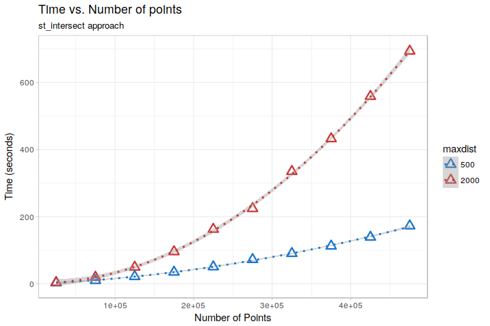
## 10: 10, 1763, 15291, 31088, 37014However, this starts to have problems over really large datasets, because the total number of comparisons to be done still rapidly increase besides the use of spatial indexes. A test done by changing the number of points in the above example in the range 25000 - 475000 shows for example this kind of behavior, for two different values of maxdist (500 and 2000 m):

On the test dataset, the relationships are almost perfectly quadratic (due to the uniform distribution of points). Extrapolating them to the 12 Million points dataset of the OP, we would get an execution time of about 14 hours for maxdist = 500, and a staggering 3.5 days formaxdist = 2000. Still doable, but not ideal…
My suggestion to the OP was therefore to “split” the points in chunks based on the x-coordinate and then work on a per-split basis, eventually assigning each chunk to a different core within a parallellized cycle.
In the end, I got curious and decided to give it a go to see what kind of performance improvement it was possible to obtain with that kind of approach. You can find results of some tests below.
A (possible) solution: Speeding up computation by combining data.table and sf_intersect
The idea here is to use a simple divide-and-conquer approach.
We first split the total spatial extent of the dataset in a certain number of regular quadrants. We then iterate over the quadrants and for each one we:
- Extract the points contained into the quadrant and apply a buffer to them;
- Extract the points contained in a slightly larger area, computed by expanding the quadrant by an amount equal to the maximum distance for which we want to identify the “neighbors”;
- Compute and save the intersection between the buffered points and the points contained in the “expanded” quadrant.
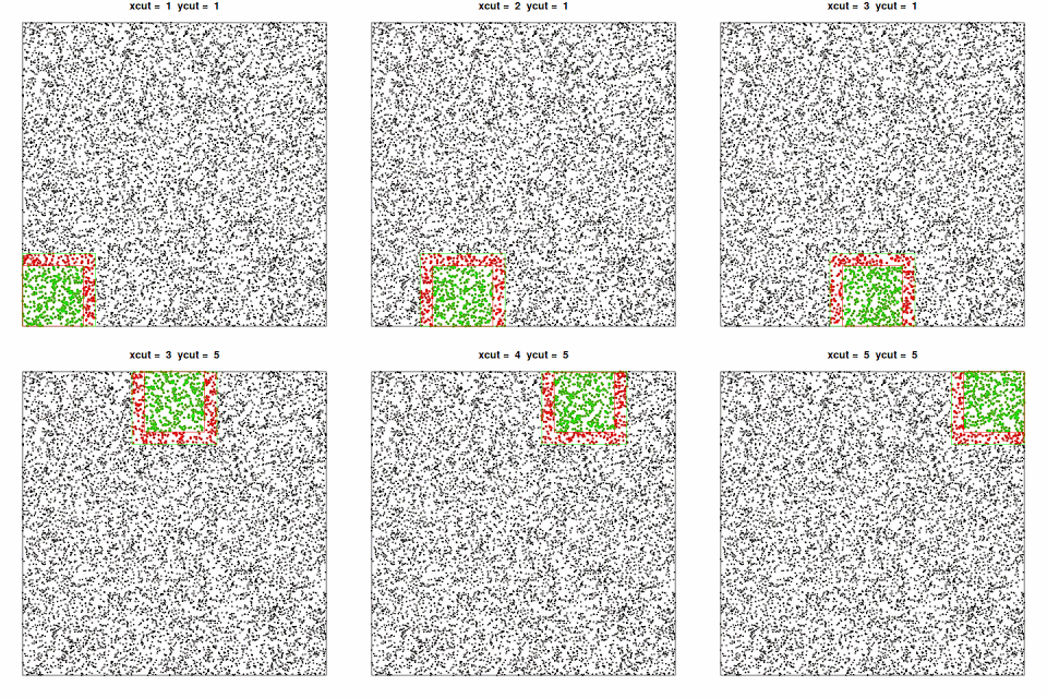
“Graphically”, this translates to exploring the dataset like this:

, where the points included in the current “quadrant” are shown in green and the additional points needed to perform the analysis for that quadrant are shown in red.
Provided that the subsetting operations do not introduce an excessive overhead (i.e., they are fast enough…) this should provide a performance boost, because it should consistently reduce the total number of comparisons to be done.
Now, every “R” expert will tell you that if you need to perform fast subsetting over large datasets the way to go is to use properly indexeddata.tables, which provide lightning-speed subsetting capabilities.
So, let’s see how we could code this in a functions:
points_in_distance <- function(in_pts,
                               maxdist,
                               ncuts = 10) {

  require(data.table)
  require(sf)
  # convert points to data.table and create a unique identifier
  pts <-  data.table(in_pts)
  pts <- pts[, or_id := 1:dim(in_pts)[1]]

  # divide the extent in quadrants in ncuts*ncuts quadrants and assign each
  # point to a quadrant, then create the index over "x" to speed-up
  # the subsetting
  range_x  <- range(pts$x)
  limits_x <-(range_x[1] + (0:ncuts)*(range_x[2] - range_x[1])/ncuts)
  range_y  <- range(pts$y)
  limits_y <- range_y[1] + (0:ncuts)*(range_y[2] - range_y[1])/ncuts
  pts[, `:=`(xcut =  as.integer(cut(x, ncuts, labels = 1:ncuts)),
             ycut = as.integer(cut(y, ncuts, labels = 1:ncuts)))]  %>%
    setkey(x)

  results <- list()
  count <- 0
  # start cycling over quadrants
  for (cutx in seq_len(ncuts)) {

    # get the points included in a x-slice extended by `maxdist`, and build
    # an index over y to speed-up subsetting in the inner cycle
    min_x_comp    <- ifelse(cutx == 1,
                            limits_x[cutx],
                            (limits_x[cutx] - maxdist))
    max_x_comp    <- ifelse(cutx == ncuts,
                            limits_x[cutx + 1],
                            (limits_x[cutx + 1] + maxdist))
    subpts_x <- pts[x >= min_x_comp & x < max_x_comp] %>%
      setkey(y)

    for (cuty in seq_len(ncuts)) {
      count <- count + 1

      # subset over subpts_x to find the final set of points needed for the
      # comparisons
      min_y_comp  <- ifelse(cuty == 1,
                            limits_y[cuty],
                            (limits_y[cuty] - maxdist))
      max_y_comp  <- ifelse(cuty == ncuts,
                            limits_y[cuty + 1],
                            (limits_y[cuty + 1] + maxdist))
      subpts_comp <- subpts_x[y >= min_y_comp & y < max_y_comp]

      # subset over subpts_comp to get the points included in a x/y chunk,
      # which "neighbours" we want to find. Then buffer them by maxdist.
      subpts_buf <- subpts_comp[ycut == cuty & xcut == cutx] %>%
        sf::st_as_sf() %>%
        sf::st_buffer(maxdist)

      # retransform to sf since data.tables lost the geometric attrributes
      subpts_comp <- sf::st_as_sf(subpts_comp)

      # compute the intersection and save results in a element of "results".
      # For each point, save its "or_id" and the "or_ids" of the points within "dist"
      inters <- sf::st_intersects(subpts_buf, subpts_comp)

      # save results
      results[[count]] <- data.table(
        id = subpts_buf$or_id,
        int_ids = lapply(inters, FUN = function(x) subpts_comp$or_id[x]))
    }
  }
  data.table::rbindlist(results)
}
The function takes as input a points sf object, a target distance and a number of “cuts” to use to divide the extent in quadrants, and provides in output a data frame in which, for each original point, the “ids” of the points within maxdist are reported in the int_ids list column.
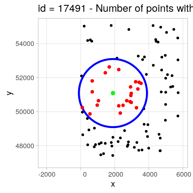
Now, let’s see if this works:
pts <- data.frame(x = runif(20000, 0, 100000),
                  y = runif(20000, 0, 100000),
                  id = 1:20000) %>%
  st_as_sf(coords = c("x", "y"), remove = FALSE)
maxdist <- 2000
out <- points_in_distance(pts, maxdist = maxdist, ncut = 10)
head(out)
## id int_ids
## 1: 5830 5830, 9068,10102, 5782,10062, 1188,...
## 2: 9068 5830, 9068,10102, 5782, 1188,15701,...
## 3: 10102 5830, 9068,10102, 5782,10062, 1188,...
## 4: 5989 5989, 7085,18143, 209, 5751, 5130,...
## 5: 5782 5830, 9068,10102, 5782,10062, 1188,...
## 6: 10062 5830,10102, 5782,10062,17566,15701,...# get a random point
sel_id <- sample(pts$id,1)
pt_sel <- pts[sel_id, ]
pt_buff <- pt_sel %>% sf::st_buffer(maxdist)
# get ids of points within maxdist
id_inters <- unlist(out[id == sel_id, ]$int_ids)
pt_inters <- pts[id_inters,]
#plot results
plot <- ggplot(pt_buff) + theme_light() +
geom_point(data = pts, aes(x = x, y = y), size = 1) +
geom_sf(col = "blue", size = 1.2, fill = "transparent") +
geom_sf(data = pt_inters, col = "red", size = 1.5) +
geom_point(data = pt_sel, aes(x = x, y = y), size = 2, col = "green") +
xlim(st_bbox(pt_buff)[1] - maxdist, st_bbox(pt_buff)[3] + maxdist) +
ylim(st_bbox(pt_buff)[2] - maxdist, st_bbox(pt_buff)[4] + maxdist) +
ggtitle(paste0("id = ", sel_id, " - Number of points within distance = ",
length(id_inters)))
plot
So far, so good. Now, let’s do the same exercise with varying number of points to see how it behaves in term of speed:

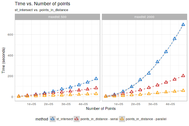
Already not bad! In particular for the maxdist = 2000 case, we get a quite large speed improvement!
However, a nice thing about the points_in_distance approach is that it is easily parallelizable. All is needed is to change some lines of the function so that the outer loop over the x “chunks” exploits a parallel backend of some kind. (You can find an example implementation exploiting foreach in this gist)
On a not-particularly-fast PC, using a 6-cores parallelization leads to this:

Looking good! Some more skilled programmer could probably squeeze out even more speed from it by some additional data.table magic, but the improvement is very noticeable.
In terms of execution time, extrapolating again to the “infamous” 12 Million points dataset, this would be what we get:
| Method | Maxdist | Expected completion time (hours) |
|---|---|---|
| st_intersect | 500 | 15 |
| points_in_distance - serial | 500 | 2.5 |
| points_in_distance - parallel | 500 | 0.57 |
| st_intersect | 2000 | 85 |
| points_in_distance - serial | 2000 | 15.2 |
| points_in_distance - parallel | 2000 | 3.18 |
So, we get a 5-6X speed improvement already on the “serial” implementation, and another 5X thanks to parallelization over 6 cores! On themaxdist = 2000 case, this means going from more than 3 days to about 3 hours. And if we had more cores and RAM to throw at it, it would finish in minutes!
###Nice!
##Final Notes
The timings shown here are merely indicative, and related to the particular test-dataset we built. On a less uniformly distributed dataset I would expect a lower speed improvement.
Some time is “wasted” because sf does not (yet) extend data.tables, making it necessary to recreate sf objects from thedata.table subsets.
The parallel implementation is quick-and-dirty, and it is a bit of a memory-hog! Be careful before throwing at it 25 processors!
Speed is influenced in a non-trivial way by the number of “cuts” used to subdivide the spatial extent. There may be a sweet-spot related to points distribution and maxdist allowing reaching maximum speed.
A similar approach for parallelization could exploit repeatedly “cropping” the original sf points object over the extent of the chunk/extended chunk. The data.table approach seems however to be faster.
That’s all! Hope you liked this (rather long) post!